R Tutorial, Day 1: Basic calculations and graphs
Written by Kim Nicholas, Klara Winkler, & Geneviève Boisjoly;
modified from Dan Kramer, Michigan State
Learning Objectives:
- Become familiar with the working environment of R, including the console, graphics device, and using scripts.
- Understand how to use functions in R.
- Import datasets into R.
- Create objects and plots in R, and be able to export them as files to your computer.
Tutorial Overview
Dataset: hpi.csv
0. Special keyboard signs in R
- R Coding and basic functions
- Importing data
- Visualizing data and plotting (histogram, plot and customization)
- Exporting graphs
- Quitting (saving)
Before starting with the R tutorial, please familiarize yourself with the following symbols - this will help you to deal with R once you have started. R uses these symbols for specific meanings, noted below.
As keyboards vary depending on your laptop and on your language, please figure out how to type the following signs on your computer and note it below. (Or you can copy and paste the symbols from here into a script and use them there.) On a Swedish keyboard, you will enter alt + 4 for $, alt + ( for [, and alt + ) for ].
$ Specifies a column name within a dataframe = Sets the value on the left equal to the value
on the right (renames, overwrites existing data!)
[ Bracket; specifies the beginning of an element of a set ] Specifies the end of an element of a set
( Parenthesis; Specifies the start of a function or argument ) Specifies the end of a function or argument
esc escape key: use to get back to main cursor prompt > NA means data are missing (different than zero)
/ Division sign * Multiplication sign ~ Tilde, used for lattice functions (Day 2-3)
Please download the following files that we’ll be using today from Live@Lund:
1. R Refcard. A handy sheet with lots of commands we’ll use in R.
2. The data file we’ll be using, „hpi.csv“. (Note: to avoid problems, do not try to open this file in Excel or another program).
3. „ScriptDay1.R“, a script file we’ve created to get you started.
1. R-CODING AND BASIC FUNCTIONS
R Coding and Script File
In order to get the most out of this tutorial, please note the following. We will present instructions and important notes in boxes such as the one around this text. We will also provide comments on what you are about to do. Therefore, below the boxes are lines of code that you enter into R (on the left) with some explanation of what you are doing on the right (after the # sign). Occasionally, we will give you task to complete. These also will be given in boxes with the title, TASK.
Before you start any R session, you should open up a script file in R (file->new script in R64, or file -> new -> R script in RStudio.)
For the tutorial 1, we started an R script for you. Download the script file R tutorial-Day 1 from Live@Lund and open it in R. Follow the first instructions in the script.
You should then type the commands below into the script (modifying as needed), and SAVE IT early and often (there is no Auto Save in R!). The name of scripts with unsaved material appear in red in RStudio. The script is what allows you to easily recreate your work, and can be built on over time (for example, saving you time in tomorrow’s exercise). Commonly, rather than saving the output, you save the recipe for producing the output in a script, so it can be instantly recreated later, as well as modified and reused. (You can also save the output, e.g., plots, directly).
Be sure to add your own comments (preceded by #) to document your work and explain it to yourself as needed.
N. B. You can send commands in the script directly to the console by pressing Command + Enter while the cursor is on a line with a command in the script.
R as Calculator
R can be used as a calculator. Note the use of # below. The # sign is used to write notes to yourself that R ignores. The order of execution of mathematical functions obeys usual mathematical rules. Type in the following commands in your R script, then run them. (You can either ignore the notes after the # sign, or include them and R will ignore them). You have to enter the coding exactly as you see it. It is caps sensitive (so: FOO, Foo, and foo are treated as different objects).
5 + 5 + 5 #You do not have to use spaces – 5+5+5 would work
7 * 10 / 2
sqrt(25) #sqrt is called a function in R. The number in the parentheses are the target of the function
Assigning Values in R
You can assign names to single values, lists of values, plots, and more complicated mathematical functions in R. (By the way, this is what is referred to as “object-oriented programming.”) Below we create a variable, x, and assign a number to it, and a list of numbers to y. Type or paste in the following assignments in your script, then run them. Remember that R is case sensitive. Note – for assignments, you can either use = or <-
x = 12 #The object x now holds the value 12.
y = c(1,2,3,4,5,6,7,8,9,10) #The c function concatenates (joins together) these numbers #in a list.
x #Typing x returns the value of 12.
y #Typing y returns the list of values 1 to 10.
Basic Statistical Functions
The power of R is really in its statistical and graphing capabilities. Try the basic functions below on the data we have already created – y.
mean(y) #Finds the mean
median(y) #Finds the median, the number exactly in the middle of the data set
range(y) #Finds the range (highest and lowest value)
min(y) #Finds the minimum
max(y) #Finds the maximum
sd(y) #Finds the standard deviation
var(y) #Finds the variance
quantile(y) #Returns values for which 25, 50, 75, and 100% of values fall below.
summary(y) #Returns the min., 1st quartile, median, mean, 3rd quartile, and max.
2. IMPORTING DATA
Importing Data
You can import data into R from a spreadsheet (e.g., MS Excel) or a text file. Today we will use a data file created by Dan Kramer at Michigan State University from the Happy Planet Index, a “leading global measure of sustainable well-being” (www.happyplanetindex.org), which uses national data on GDP and alternative measures of productivity and happiness.
The trickiest part is figuring out how to tell R where to look on your computer to find the file you want. We’ll start by finding out where R is looking by default, and create a folder there to put the files we want to read into R.
Download the file called “hpi.csv” from Live@Lund and follow directions below to put it in a place on your computer where R can access it. To avoid problems, don’t open this file with Excel or any other programs on your computer.
We’ll practice what you have learned so far using this data set. A list of variable names and their descriptions are below; read this carefully so that you understand what you are plotting. You refer to the “Variable Name” when coding in R.
Variable name
Description
code
3-letter country code- useful for labeling points on a plot
country
Full country name
region
Geographical region, expressed numerically. The number is broad region (e.g., 1= North and South America) and the letter is a smaller region (e.g., 1a = Central America; 1b= South America). These are not that useful- we have added columns at the end with region names.
lifesat
This is “experienced well-being,” taken from a Gallup World Poll where respondents answer a survey question assessing their life satisfaction on a scale from 1 (low) to 10 (high).
lifeexp
Average years of life expectancy, from the 2011 UNDP Human Development Report
footprint
“The HPI uses the Ecological Footprint promoted by the environmental charity WWF as a measure of resource consumption. It is a per capita measure of the amount of land required to sustain a country’s consumption patterns, measured in terms of global hectares (g ha) which represent a hectare of land with average productive biocapacity.” http://www.happyplanetindex.org/about/
The HPI takes an Ecological Footprint of 1.78 g ha per capita as the equivalent of “one-planet living” (above this represents overconsumption).
hly
A weighted index of Happy Life Years, approximated by: (lifeexp * lifesat)/100. This measure discounts life expectancy based on happiness.
hpi
According to its creators, “The HPI measures what matters. the extent to which countries deliver long, happy, sustainable lives for the people that live in them.”
http://www.happyplanetindex.org/about/
The calculation shown is approximate (squiggly equals sign) because the authors make certain statistical adjustments- see p. 20-21 of the appendix of the full report for details.
The creators of the Happy Planet Index state, “On a scale of 0 to 100 for the HPI, we have a target for nations to aspire to by 2050 of 89. This is based on attainable levels of life expectancy and well-being and a reasonably-sized Ecological Footprint.” See more at: http://www.happyplanetindex.org/about/#sthash.ucoVoSqw.dpuf
hpirank
A ranked order of the top country (1) to the lowest (143), based on HPI scores.
gdpcap
Gross Domestic Product per capita, a standard measure of national economic performance. Units: US Dollars $ per person.
hdi
Human Development index. A measure used by the United Nations Development Programme to quantify national human development potential using measures of life expectancy, education, and income. Here expressed as a decimal on a scale from 0 (low) to 1 (high).
pop
National population (number of people).
region.names
These are region names added by Kim based on the existing region labels in the data, to make interpretation easier. There are 15 options: CentAm, SAm, AustNZ, NAm, Eur, MENA, CentAfr, EastAfr, WestAfr, SAsia, EastAsia, SEAsia, CentAsia, EastEur, Soviet
big.regions
These are labels added by Kim to put all countries into one of only four very broad categories: Americas, Asia, Europe, and Africa. This is for broad-scale comparisons.
Brief meta-data is available here: http://www.happyplanetindex.org/about/
Full meta-data: http://www.happyplanetindex.org/assets/happy-planet-index-report.pdf , p. 19-21
#PUT DATA WHERE R CAN FIND THEM
#OPTION 1: THE EASY WAY (MAC)
# create a folder on your computer where you want to store your R data files. Say you have an ESS folder already- then you create a folder called “methods” within the ESS folder, then a folder called “datafiles” within the methods folder (best not to use spaces).
# Place the “hpi.csv” file within the “methods” folder.
MAC
# Click once on the .csv-filepress and then the Command key (⌘) + I to pull up the information window.
# In the “where” box, the filepath to the hpi.csv file will be shown: “/Users/kanicholas/ESS/methods/datafiles”
Windows
# Click once on the .csv-file and then in the command line
# The filepath to the hpi.csv-file will be shown: “C: \ESS folder\methods\datafiles”
# paste this filepath in the script where you read in the data
Windows
# Change the backslashes to forwards slashes (\ à /)
#OPTION 2: THE SLIGHTLY LESS EASY WAY (MAC AND PC)
getwd() #then press Return to run the command
# tells you where your working directory is. In other words, where will R look for
# files? It will return something like this:
#[1] "/Users/kanicholas" for Mac (note filepaths are always forward slashes)
#[1] "C:/Documents and Settings/tkrau" for PC
# The location shown here (e.g., within the folder “kanicholas”) is where you want to create a folder called "methods" (all lower case).
# you can create sub-folders within this folder to organize your files
# for now, put the "hpi.csv” file from the website in the “methods” folder.
# so in the example above, I would create a folder called “methods” within the “kanicholas” folder on my computer, which is within the “users” folder. I then put the “hpi.csv” file in this “methods” folder. Make sure the file format is listed (e.g., the file is called “hpi.csv” rather than just “hpi”.
# Once you’ve placed the data file where R will look for it, you can read in the data.
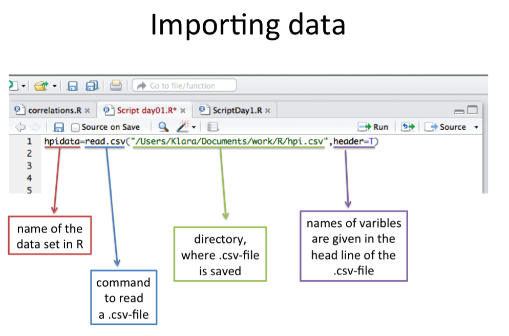
hpidata=read.csv("/Users/kanicholas/methods/hpi.csv",header=TRUE)
# this is what Kim uses to access the data on her hard drive. Replace the part underlined in bold with your own filepath (cut and paste the result returned by the “getwd()” command or the Command + I exercise). Make sure you have used forward slashes before/after parts as above, and specified the filename (hpi.csv) as the last item.
#Now that you’ve read in the data, inspect it.
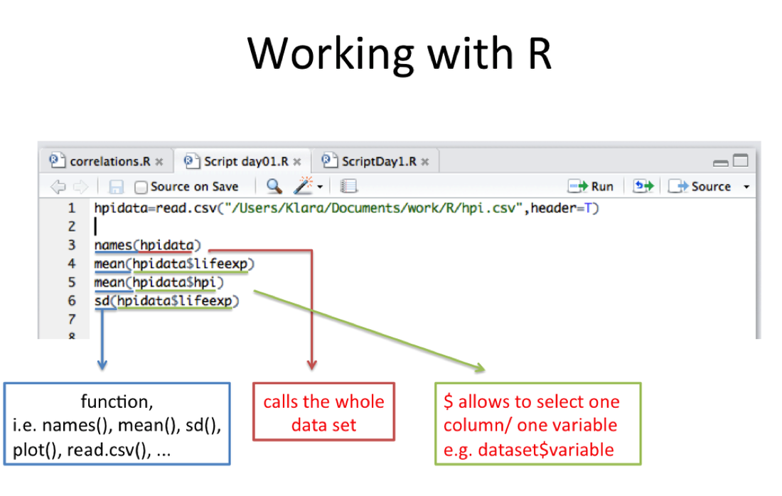
hpidata #Typing the name of an object displays it in full- this shows the data you just imported.
View(hpidata) #A snazzy way to look at a spreadsheet version of the data. Note the “V” is capitalized.
names(hpidata) #Shows you all the variable names. Remember, refer to the list above for what they mean.
hpidata$gdpcap #returns values in the column named "gdpcap"
hpidata[,1] #returns all rows, first column
hpidata[1,] #returns first row, all columns
hpidata[1,1] #returns the value in the first row, first column. Since this is a factor, it lists all the levels found here.
hpidata[1:3,1:2] #returns first three rows, first two columns
dim(hpidata) #dimensions of data (first number of rows, then number of columns)
head(hpidata) #shows the first few lines of the data
tail(hpidata) #shows the last few lines of the data
class(hpidata) #tells you what kind of object “hpidata” is.
sapply(hpidata, class) #tells you what kind of variable each column in “hpidata” is. Some possible types include strings (characters, such as names), factors (levels of a treatment), or numbers such as integers or numeric.
class(hpidata$pop) # R reads in “pop” as integer (a whole number with no decimals). We want to make it a “numeric” class so we can work with it in operations.
hpidata$pop= as.numeric(hpidata$pop) # We have reassigned the class of the column “pop” from integer to numeric.
class(hpidata$pop) # Should now read “numeric” after our re-assignment.
hpidata$gdp=hpidata$gdpcap *hpidata$pop #We create a new column called “gdp,” total national GDP, which we calculate by multiplying the two columns (hpidata$gdpcap*hpidata$pop).
head(hpidata) #check the values for the new column, “gdp”.
write.csv(hpidata,"/Users/kanicholas/methods/hpi2.csv")
# since we have modified the original hpidata file, if we want to keep our changes (new gdp column) we should save it with a new name. Replace the underlined part in the command above with your filepath from before. The last part of the filepath will be the name for the file you create (now hpi2 instead of hpi). You can read in this file in the future to work with the data. Remember to always keep an original copy of all data files before you did any modifications (save any changes you make in R with a new file name, so you have the original “hpi.csv” to go back to).
TASK 1
Find the mean, median, and standard deviation for the variables Life Expectancy in Years (lifeexp) and Happy Life Years (hly). For what age do 50% of the countries fall below? How about 75%?
Add a new column to hpidata: Calculate the total country footprint (call it “totalfoot”, footprint in hectares) for the entire national population (pop). Inspect the data. Which country is highest? Which country is lowest?
# SAVE YOUR SCRIPT FILE!!
3. VISUZALIZING & PLOTTING DATA
Graphs
One of the more appealing capabilities of R is its endless plotting capabilities. Below are a few of the most popular plotting functions: histograms, plots and scatterplots, and boxplots. R offers countless ways to customize graphics.
Histogram (R code: hist)
A histogram shows distributions of data. The frequency indicates what proportion of the data falls in each category. This is a good graph to make early on when you are getting a sense of your data.
hist(hpidata$gdpcap) #Plots a histogram or distribution of the values of gdpcap.
hist(hpidata$gdpcap, breaks=4) #Specify the number of bins you want to group the data into.
hist(hpidata$gdpcap, main="Distribution of national GDP/capita") #Assign a title to your graph.
hist(hpidata$gdpcap,main="Distribution of national GDP/capita",xlab="GDP/cap ($/capita)")
#Assign a label for the x-axis.
hist(hpidata$gdpcap,main="Distribution of national GDP/capita",xlab="GDP/cap ($/capita)",col="red")
#Add color
# SAVE YOUR SCRIPT FILE!!
TASK 2
Plot a histogram of another variable of hpidata (you will have to select a numeric variable to plot). For this plot, add a title, an x-axis label, a y-axis label, and color, and select the number of bins to appropriately represent the data. Show us your results when you are done and explain what they mean.
Plots and Scatterplot (R code: plot & lines)
Perhaps the most basic plot. This function simply plots data points. You can plot individual variables or pairs of variables (i.e., scatterplots). We’ll do both below.
plot(hpidata$footprint) #Plots the values of y according to its position in the list.
lines(hpidata$footprint) #Same but connects the dots with a line. Not meaningful in this case, where there is no connection between one country and the next, but good for timeseries data.
plot(hpidata$gdpcap,hpidata$footprint) #Plots the paired values for x and y.
# SAVE YOUR SCRIPT FILE!!
TASK 3
Add a meaningful title, x label, y label, and a new color to your last graph. To see a list of all 655 color names in R, type colors().
Further Customizing Graphics
Below are a number of different functions you can use to customize the graphics that you create in R. We’ll use the plot function to look at the relationships of a few variables in our dataset hpidata.
plot(hpidata$lifesat, hpidata$gdpcap) #xyplot of these two variables.
# Hm, we’d like to know which points belong to which countries. To do this, we can first plot the data with just a small point for each country, then follow with the text() function which will overlay names on the points we’ve already plotted.
plot(hpidata$lifesat, hpidata$gdpcap, pch=".") #xyplot with small points.
text(hpidata$lifesat, hpidata$gdpcap, hpidata$code, cex=0.5, pos=2, col="red")
#at the xy coordinates specified by the first two terms, add the label "code". You can follow any of the next commands with this to label the points.
plot(hpidata$lifesat, hpidata$gdpcap, xlim=c(4,8)) #Limit the length of the x-axis
plot(hpidata$lifesat, hpidata$gdpcap, ylim=c(0,30000))#Limit the length of the y-axis
plot(hpidata$lifesat, hpidata$gdpcap, pch=20) #Change how points are plotted (1 to 21). “1” is the default. Try changing the number.
plot(hpidata$lifesat, hpidata$gdpcap, cex=2) #Make points larger. “1” is default
plot(hpidata$lifesat, hpidata$gdpcap, bty="n") #Determines kind of box around plot. Choices are o,l, 7, c, u, n, and ]. Try them.
plot(hpidata$lifesat, hpidata$gdpcap, col.axis="red") #Changes color of axis labels
plot(hpidata$lifesat, hpidata$gdpcap, col.lab="green")#Changes color of x & y labels
plot(hpidata$lifesat, hpidata$gdpcap, main="GDP/capita vs. Lifesatisfaction", col.main="purple") #Title color
plot(hpidata$lifesat, hpidata$gdpcap, font=2) #Change the font from 1 (default) to 5. Can also use font.axis, font.lab, font.main as you did with color. Try it.
plot(hpidata$lifesat, hpidata$gdpcap, las=2) #Changes the orientation of axis labels from 0 (default) to 3. Try it.
# SAVE YOUR SCRIPT FILE!!
TASK 4
What is the relationship between life expectancy (lifeexp) and ecological footprint (footprint)? Use the plot function to show the relationship graphically. Use each of the above options (i.e., pch, cex, font, las etc.) to create a highly customized graphic. Discuss what you see with a neighbor. Show us the graphic when you are finished and explain what it means.
4. Exporting & Consolidating Graphs
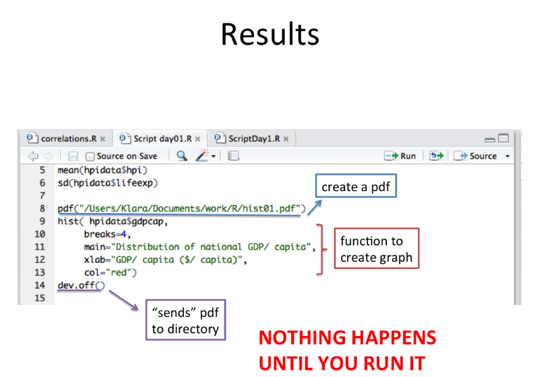
Given the great graphing capabilities of R, you want to be able to export graphs for use in papers and presentations. Below, we show you how to do this in several different formats. After creating the plots, be sure to open the “methods” folder on your computer to look at them. Note that these three commands - pdf(), plot(), and dev.off()- must be called in order before the plot appears in the “methods” folder- it will look like nothing has happened until you call dev.off().
pdf("/Users/kanicholas/methods/plot1.pdf") #Export next plot as pdf with file name “plot1.pdf” to the directory specified before the last slash. Change the part in bold to your own directory.
plot(hpidata$lifesat, hpidata$gdpcap, las=2) #Replace the italicized command with the script for the specialized plot you made above.
dev.off() #R releases the plot for export. File appears as a PDF in the specified folder. Nothing goes within the parentheses here.
# Note : A common problem is that you have called a new graphics device, such as pdf() or jpg(), without turning it off. Then it will appear as if your plots are not being created, because they are being sent to a pdf printer but not printed. If this is happening, you can use
dev.cur() #tells you what the current graphics device is. If it is something like pdf or jpg, use this command:
dev.off() # this turns off the phantom graphing device. Try calling the plot again, it should now appear in the default plotting window. If not, you can use:
dev.new() #to make a new plotting window appear.
tiff("/Users/kanicholas/methods/plot2.tif") #Export next plot a tif
plot(hpidata$lifesat,hpidata$gdpcap, las=2) #replace italicized script with your plot command
dev.off()
jpeg("/Users/kanicholas/methods/plot3.jpeg") #Export next plot as jpeg
plot(hpidata$lifesat,hpidata$gdpcap, las=2) #Replace italicized script with your plot command
dev.off()
pdf("/Users/kanicholas/methods/multiplot.pdf") #Consolidated 3 plots as pdf
par(mfrow=c(3,1)) #3 graphs in 3 rows and 1 column
plot(hpidata$lifeexp, hpidata$footprint, pch=19,col="blue")
plot(hpidata$lifesat, hpidata$lifeexp, pch=18,col="orange")
plot(hpidata$gdpcap, hpidata$hdi, pch=17,col="darkgreen")
par(mfrow=c(1,1)) #reset to default, one plot per screen
dev.off()
5. Quitting R and saving
Before quitting R, save your script file. Upon quitting R, you are asked if you would like to save the workspace. The workspace is the list of all the scripts you used in this particular session. Say YES.
q() #Exit from R

R Tutorials by Kimberly A. Nicholas is licensed under a Creative Commons Attribution-NonCommercial-ShareAlike 4.0 International License.